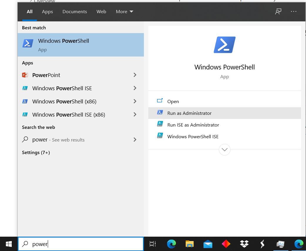
Open PowerShell as Administrator:
CDO installation and use
1. From the CDO documentation
2. Install wsl
2.1. Option #1:
2.2. Option #2
2.3. Update to WSL 2 (check Windows version)
2.4. Enable Virtual Machine feature
2.5. Download the Linux kernel update package
2.6. Set WSL 2 as your default version
2.7. Install Linux distro
Open the Microsoft Store and select a Linux distribution (distro)
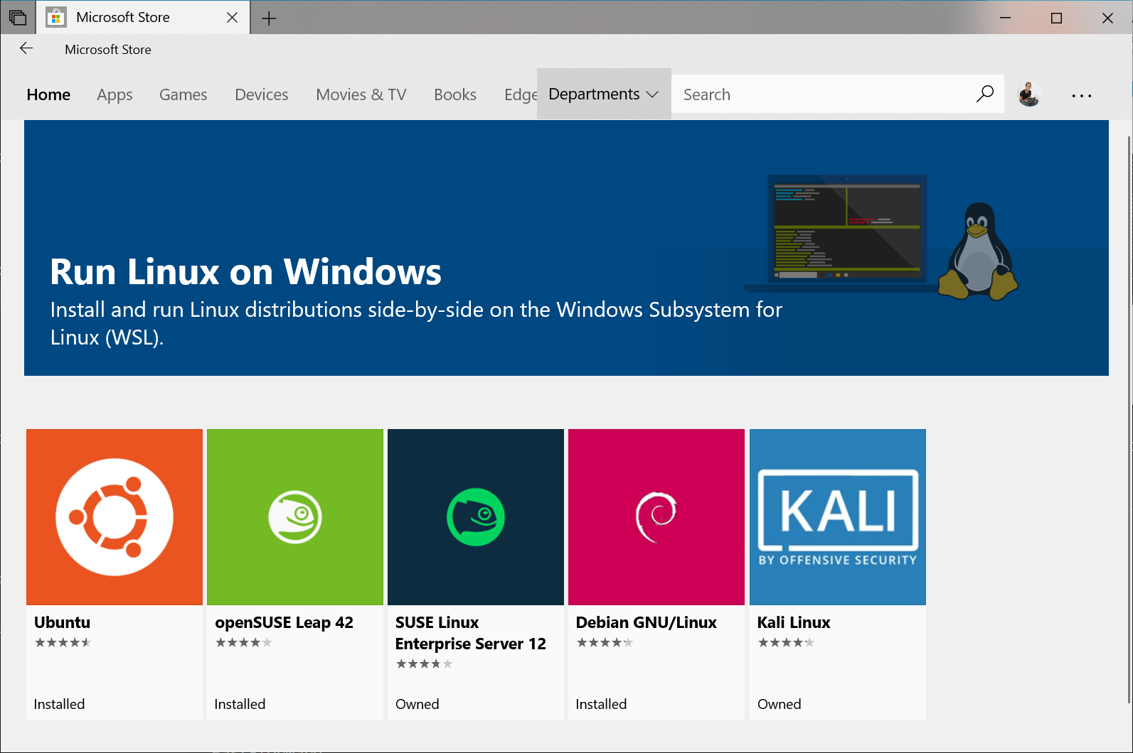
Ubuntu 18.04 and 20.04 were tested for CDO. After this, Ubuntu
should be a searchable program in Windows
3. Setting up Ubuntu
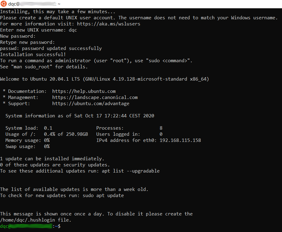
Open the Ubuntu app
On the first lunch, it will show this:
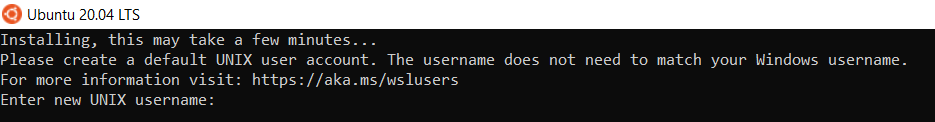
Set credentials, user and password (twice)
Output should look like this:
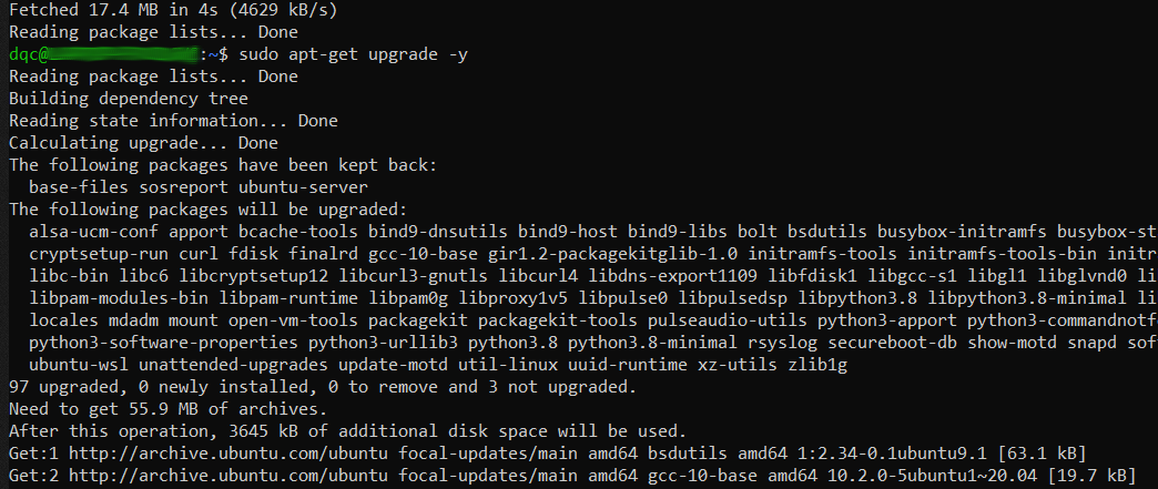
3.2. Update and upgrade
4. Install and check CDO
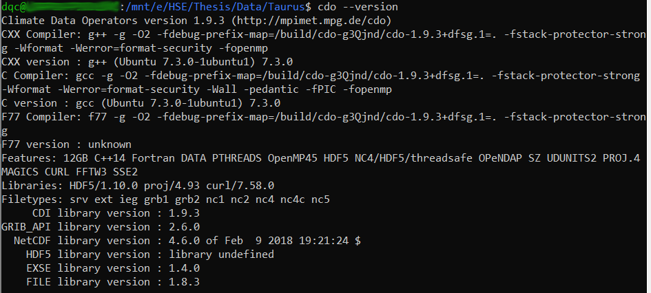
4.1. CDO version
Check that CDO is working with:
cdo --version
5. CDO installation in MacOS
6. Basic shell commands
7. Accessing Windows files from Linux
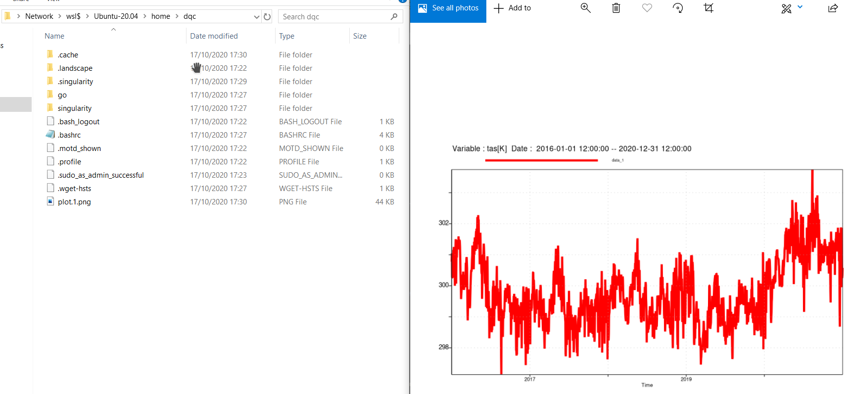
8. Accessing Linux files from Windows
Type
\\wsl$on the file explorer path (on the top), enterThen click Ubuntu → home → user
Should look something like this (note the plot created before):
9. Exercise
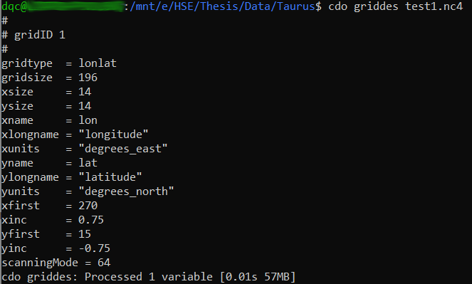
10. Exploration
11. Visualization
11.1. 2D Lon-Lat

11.3. Line graph plots

12. Manipulation of files
12.1. Merge
12.2. Cropping
12.3. Exporting to text
13. Downloading CORDEX files
Create account for ESGF node
Login with your
OpenIDafter receiving confirmation emailRegister to the CORDEX group
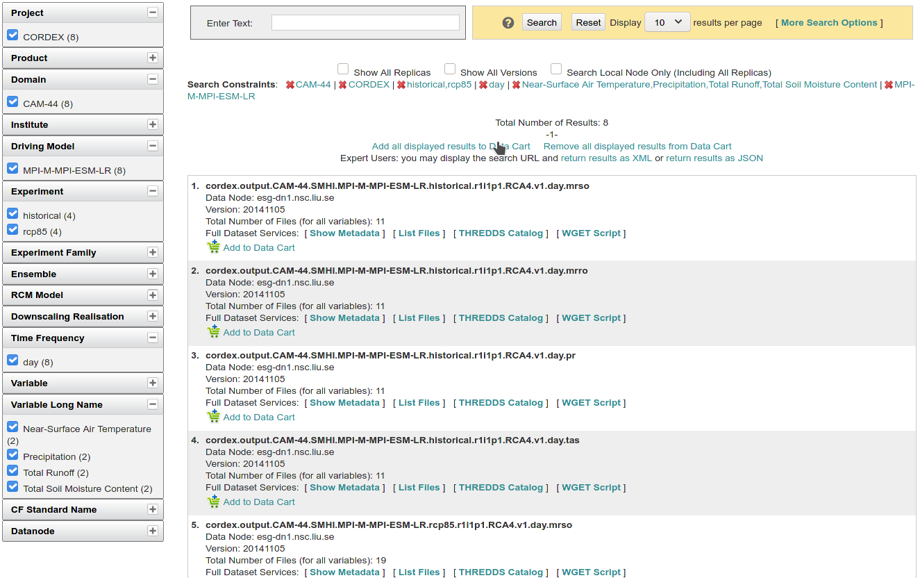
Explore and select desired data (checked boxes, note for later, where the pointer is)
13.1. File by file
To download file by file through your browser click on
list filesThen click on
HTTP Download, this will open a prompt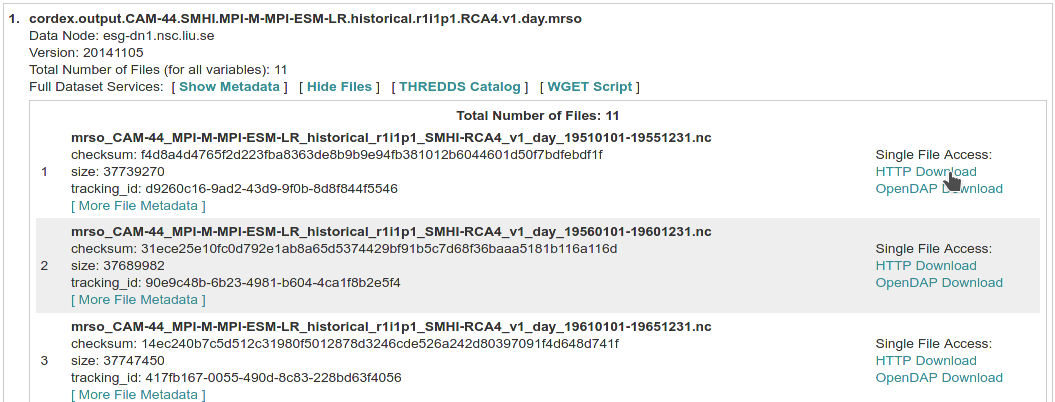
Save file and repeat
Note that CORDEX files are usually on a 5 years basis (daily)
13.2. The automated way
Click on
Add all displayed results to Data Cart(where the
pointer was in the penultimate image)Go to your
data cart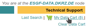
Select datasets to download. When ready, click on
WGET Script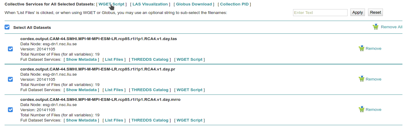
Depending on your dataset, there might be several
WGET Scripts.
Click and save them.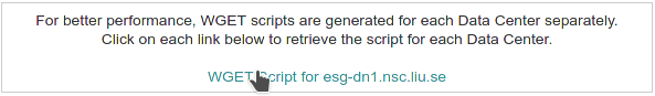
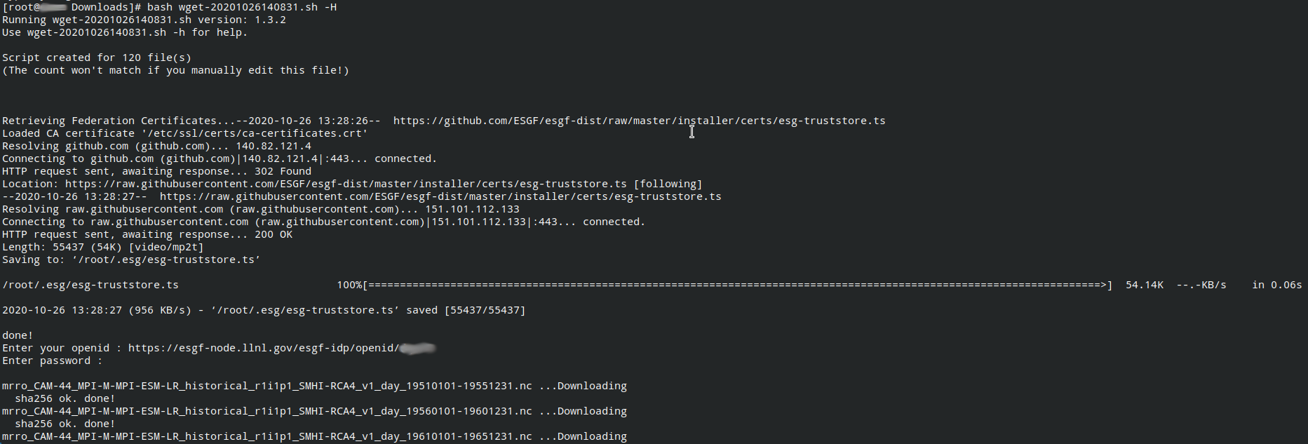
13.3. Run script
Open a Linux terminal
Go to your downloads folder (see point 7)
Run the following command (change the name appropriately):
bash wget-20201026140831.sh -H
# The -H is to interactively enter your credentials
Give credentials, the full
OpenIDlooks like:
https://esgf-node.llnl.gov/esgf-idp/openid/userThis will start the download process of the
NetCDFfilesThis process will take a while and should look like this: